If Subjects Become Available Again will They Be Included in Survival Analysis

Branch of statistics

Survival analysis is a branch of statistics for analyzing the expected duration of time until one event occurs, such as death in biological organisms and failure in mechanical systems. This topic is called reliability theory or reliability assay in engineering, duration analysis or duration modelling in economics, and issue history analysis in sociology. Survival analysis attempts to answer certain questions, such as what is the proportion of a population which will survive past a certain time? Of those that survive, at what rate will they dice or fail? Can multiple causes of decease or failure be taken into account? How do particular circumstances or characteristics increase or decrease the probability of survival?

To reply such questions, it is necessary to define "lifetime". In the case of biological survival, death is unambiguous, but for mechanical reliability, failure may not exist well-defined, for there may well be mechanical systems in which failure is fractional, a matter of degree, or not otherwise localized in time. Even in biological bug, some events (for example, heart assault or other organ failure) may have the aforementioned ambivalence. The theory outlined below assumes well-defined events at specific times; other cases may be better treated by models which explicitly account for cryptic events.

More than by and large, survival analysis involves the modelling of time to event data; in this context, death or failure is considered an "outcome" in the survival assay literature – traditionally just a single outcome occurs for each subject, after which the organism or mechanism is dead or broken. Recurring upshot or repeated effect models relax that supposition. The written report of recurring events is relevant in systems reliability, and in many areas of social sciences and medical research.

Introduction to survival assay [edit]

Survival assay is used in several ways:

• To describe the survival times of members of a group
  • Life tables
  • Kaplan–Meier curves
  • Survival part
  • Hazard part
• To compare the survival times of two or more groups
  • Log-rank exam
• To describe the effect of categorical or quantitative variables on survival
  • Cox proportional hazards regression
  • Parametric survival models
  • Survival trees
  • Survival random forests

Definitions of common terms in survival analysis [edit]

The following terms are commonly used in survival analyses:

• Effect: Death, disease occurrence, disease recurrence, recovery, or other experience of interest
• Time: The time from the beginning of an observation period (such equally surgery or beginning handling) to (i) an upshot, or (2) end of the written report, or (iii) loss of contact or withdrawal from the report.
• Censoring / Censored observation: Censoring occurs when we have some information almost individual survival fourth dimension, just nosotros do not know the survival time exactly. The subject is censored in the sense that zero is observed or known nearly that subject after the time of censoring. A censored subject may or may not have an result after the stop of ascertainment time.
• Survival office Southward(t): The probability that a subject survives longer than time t.

Instance: Acute myelogenous leukemia survival data [edit]

This instance uses the Acute Myelogenous Leukemia survival data set "aml" from the "survival" package in R. The data set is from Miller (1997)^[i] and the question is whether the standard course of chemotherapy should exist extended ('maintained') for boosted cycles.

The aml data set sorted by survival time is shown in the box.

aml information set sorted by survival time

• Time is indicated past the variable "fourth dimension", which is the survival or censoring time
• Event (recurrence of aml cancer) is indicated by the variable "status". 0= no upshot (censored), 1= event (recurrence)
• Treatment group: the variable "x" indicates if maintenance chemotherapy was given

The last observation (11), at 161 weeks, is censored. Censoring indicates that the patient did not take an result (no recurrence of aml cancer). Another bailiwick, observation 3, was censored at xiii weeks (indicated past status=0). This field of study was in the study for only 13 weeks, and the aml cancer did not recur during those thirteen weeks. It is possible that this patient was enrolled near the end of the report, so that they could be observed for simply 13 weeks. It is too possible that the patient was enrolled early on in the report, but was lost to follow up or withdrew from the report. The table shows that other subjects were censored at 16, 28, and 45 weeks (observations 17, 6, and9 with status=0). The remaining subjects all experienced events (recurrence of aml cancer) while in the study. The question of involvement is whether recurrence occurs later in maintained patients than in non-maintained patients.

Kaplan–Meier plot for the aml data [edit]

The survival function Due south(t), is the probability that a field of study survives longer than time t. Southward(t) is theoretically a smooth curve, just information technology is normally estimated using the Kaplan–Meier (KM) curve. The graph shows the KM plot for the aml information and can exist interpreted as follows:

• The x axis is time, from zero (when observation began) to the last observed time indicate.
• The y axis is the proportion of subjects surviving. At time zero, 100% of the subjects are alive without an effect.
• The solid line (similar to a staircase) shows the progression of event occurrences.
• A vertical drop indicates an event. In the aml tabular array shown above, 2 subjects had events at five weeks, two had events at eight weeks, one had an issue at nine weeks, and then on. These events at 5 weeks, 8 weeks and so on are indicated by the vertical drops in the KM plot at those fourth dimension points.
• At the far right end of the KM plot there is a tick marking at 161 weeks. The vertical tick mark indicates that a patient was censored at this fourth dimension. In the aml data tabular array five subjects were censored, at 13, 16, 28, 45 and 161 weeks. There are five tick marks in the KM plot, corresponding to these censored observations.

Life table for the aml data [edit]

A life table summarizes survival data in terms of the number of events and the proportion surviving at each event fourth dimension signal. The life table for the aml data, created using the Rsoftware, is shown.

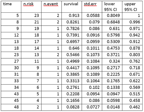
Life table for the aml data

The life table summarizes the events and the proportion surviving at each effect time point. The columns in the life table have the post-obit estimation:

• time gives the fourth dimension points at which events occur.
• n.run a risk is the number of subjects at risk immediately before the time point, t. Being "at hazard" means that the bailiwick has not had an event before time t, and is not censored before or at time t.
• n.event is the number of subjects who take events at time t.
• survival is the proportion surviving, as determined using the Kaplan–Meier production-limit gauge.
• std.err is the standard error of the estimated survival. The standard error of the Kaplan–Meier production-limit gauge information technology is calculated using Greenwood'southward formula, and depends on the number at risk (northward.risk in the tabular array), the number of deaths (due north.issue in the table) and the proportion surviving (survival in the table).
• lower 95% CI and upper 95% CI are the lower and upper 95% confidence bounds for the proportion surviving.

Log-rank test: Testing for differences in survival in the aml data [edit]

The log-rank examination compares the survival times of two or more groups. This instance uses a log-rank test for a divergence in survival in the maintained versus non-maintained treatment groups in the aml data. The graph shows KM plots for the aml data broken out by handling group, which is indicated by the variable "ten" in the information.

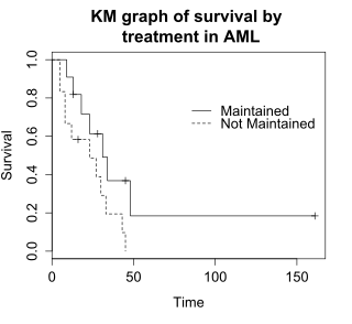
Kaplan–Meier graph by treatment group in aml

The naught hypothesis for a log-rank test is that the groups accept the same survival. The expected number of subjects surviving at each time point in each is adjusted for the number of subjects at hazard in the groups at each upshot fourth dimension. The log-rank examination determines if the observed number of events in each grouping is significantly different from the expected number. The formal test is based on a chi-squared statistic. When the log-rank statistic is large, it is prove for a deviation in the survival times between the groups. The log-rank statistic approximately has a chi-squared distribution with one degree of freedom, and the p-value is calculated using the chi-squared distribution.

For the example data, the log-rank test for difference in survival gives a p-value of p=0.0653, indicating that the treatment groups do not differ significantly in survival, assuming an alpha level of 0.05. The sample size of 23 subjects is pocket-sized, so there is piffling power to detect differences betwixt the treatment groups. The chi-squared test is based on asymptotic approximation, so the p-value should be regarded with caution for small sample sizes.

Cox proportional hazards (PH) regression analysis [edit]

Kaplan–Meier curves and log-rank tests are well-nigh useful when the predictor variable is chiselled (due east.g., drug vs. placebo), or takes a modest number of values (due east.g., drug doses 0, 20, l, and 100 mg/solar day) that can be treated as categorical. The log-rank test and KM curves don't work hands with quantitative predictors such every bit gene expression, white blood count, or age. For quantitative predictor variables, an culling method is Cox proportional hazards regression analysis. Cox PH models work also with categorical predictor variables, which are encoded as {0,i} indicator or dummy variables. The log-rank test is a special instance of a Cox PH analysis, and tin be performed using Cox PH software.

Example: Cox proportional hazards regression analysis for melanoma [edit]

This example uses the melanoma data gear up from Dalgaard Chapter xiv. ^[2]

Data are in the R package ISwR. The Cox proportional hazards regression usingR gives the results shown in the box.

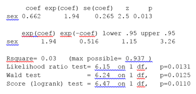
Cox proportional hazards regression output for melanoma data. Predictor variable is sex 1: female, 2: male.

The Cox regression results are interpreted as follows.

• Sex is encoded every bit a numeric vector (i: female, two: male). The Rsummary for the Cox model gives the hazard ratio (HR) for the 2d group relative to the first group, that is, male versus female.
• coef = 0.662 is the estimated logarithm of the hazard ratio for males versus females.
• exp(coef) = ane.94 = exp(0.662) - The log of the hazard ratio (coef= 0.662) is transformed to the hazard ratio using exp(coef). The summary for the Cox model gives the hazard ratio for the 2nd grouping relative to the first group, that is, male versus female. The estimated hazard ratio of ane.94 indicates that males have higher risk of death (lower survival rates) than females, in these data.
• se(coef) = 0.265 is the standard error of the log hazard ratio.
• z = 2.v = coef/se(coef) = 0.662/0.265. Dividing the coef by its standard mistake gives the z score.
• p=0.013. The p-value corresponding to z=2.5 for sexual practice is p=0.013, indicating that there is a significant divergence in survival equally a part of sex.

The summary output also gives upper and lower 95% confidence intervals for the hazard ratio: lower 95% leap = one.15; upper 95% bound = iii.26.

Finally, the output gives p-values for 3 alternative tests for overall significance of the model:

• Likelihood ratio test = 6.fifteen on i df, p=0.0131
• Wald exam = 6.24 on i df, p=0.0125
• Score (log-rank) test = half dozen.47 on one df, p=0.0110

These three tests are asymptotically equivalent. For big enough N, they will give similar results. For pocket-size N, they may differ somewhat. The last row, "Score (logrank) exam" is the result for the log-rank test, with p=0.011, the same result as the log-rank exam, considering the log-rank test is a special case of a Cox PH regression. The Likelihood ratio examination has improve beliefs for minor sample sizes, and so it is by and large preferred.

Cox model using a covariate in the melanoma data [edit]

The Cox model extends the log-rank test past allowing the inclusion of additional covariates. This example utilize the melanoma data set where the predictor variables include a continuous covariate, the thickness of the tumor (variable proper noun = "thick").

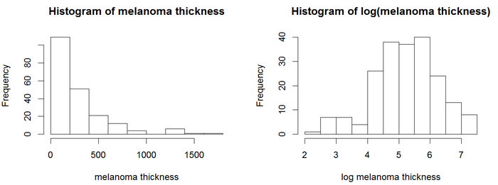
Histograms of melanoma tumor thickness

In the histograms, the thickness values don't look normally distributed. Regression models, including the Cox model, by and large give more reliable results with normally-distributed variables. For this instance employ a log transform. The log of the thickness of the tumor looks to be more normally distributed, and so the Cox models will use log thickness. The Cox PH assay gives the results in the box.

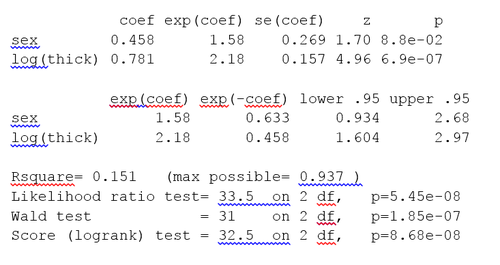
Cox PH output for melanoma information gear up with covariate log tumor thickness

The p-value for all three overall tests (likelihood, Wald, and score) are pregnant, indicating that the model is significant. The p-value for log(thick) is 6.9e-07, with a hazard ratio HR = exp(coef) = 2.18, indicating a strong relationship between the thickness of the tumor and increased risk of death.

By contrast, the p-value for sex is now p=0.088. The take chances ratio 60 minutes = exp(coef) = i.58, with a 95% conviction interval of 0.934 to ii.68. Because the confidence interval for HR includes 1, these results bespeak that sex activity makes a smaller contribution to the difference in the 60 minutes after decision-making for the thickness of the tumor, and but trend toward significance. Examination of graphs of log(thickness) past sex and a t-test of log(thickness) by sex activity both indicate that at that place is a significant departure between men and women in the thickness of the tumor when they offset encounter the clinician.

The Cox model assumes that the hazards are proportional. The proportional gamble assumption may be tested using the Rfunction cox.zph(). A p-value is less than 0.05 indicates that the hazards are not proportional. For the melanoma data, p=0.222, indicating that the hazards are, at least approximately, proportional. Additional tests and graphs for examining a Cox model are described in the textbooks cited.

Extensions to Cox models [edit]

Cox models can be extended to deal with variations on the elementary assay.

• Stratification. The subjects can be divided into strata, where subjects within a stratum are expected to exist relatively more than like to each other than to randomly chosen subjects from other strata. The regression parameters are assumed to be the same beyond the strata, but a different baseline hazard may exist for each stratum. Stratification is useful for analyses using matched subjects, for dealing with patient subsets, such as different clinics, and for dealing with violations of the proportional hazard supposition.
• Time-varying covariates. Some variables, such as gender and treatment group, more often than not stay the same in a clinical trial. Other clinical variables, such as serum protein levels or dose of concomitant medications may change over the course of a study. Cox models may be extended for such time-varying covariates.

Tree-structured survival models [edit]

The Cox PH regression model is a linear model. It is like to linear regression and logistic regression. Specifically, these methods assume that a single line, curve, aeroplane, or surface is sufficient to separate groups (alive, dead) or to estimate a quantitative response (survival fourth dimension).

In some cases alternative partitions requite more accurate classification or quantitative estimates. One set of alternative methods are tree-structured survival models,^{[three] [4] [v]} including survival random forests.^[6] Tree-structured survival models may give more accurate predictions than Cox models. Examining both types of models for a given data set up is a reasonable strategy.

Example survival tree analysis [edit]

This example of a survival tree analysis uses the Rpacket "rpart".^[7] The instance is based on 146 stageC prostate cancer patients in the data set stagec in rpart. Rpart and the stagec example are described in Atkinson and Therneau (1997),^[8] which is also distributed as a vignette of the rpart package.^[7]

The variables in stages are:

• pgtime: time to progression, or last follow-up free of progression
• pgstat: status at last follow-upward (1=progressed, 0=censored)
• age: age at diagnosis
• eet: early endocrine therapy (i=no, 0=yes)
• ploidy: diploid/tetraploid/aneuploid Dna blueprint
• g2: % of cells in G2 phase
• course: tumor form (1-four)
• gleason: Gleason grade (3-10)

The survival tree produced by the analysis is shown in the figure.

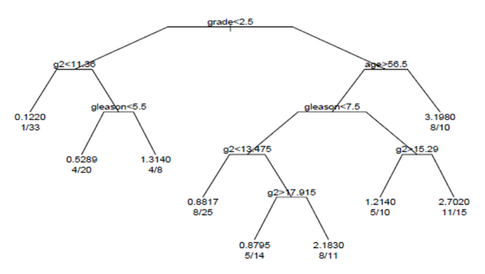
Survival tree for prostate cancer data set

Each branch in the tree indicates a split on the value of a variable. For example, the root of the tree splits subjects with grade < 2.five versus subjects with grade ii.v or greater. The terminal nodes indicate the number of subjects in the node, the number of subjects who have events, and the relative effect charge per unit compared to the root. In the node on the far left, the values ane/33 signal that ane of the 33 subjects in the node had an event, and that the relative result rate is 0.122. In the node on the far right bottom, the values 11/15 indicate that 11 of xv subjects in the node had an event, and the relative event charge per unit is 2.7.

Survival random forests [edit]

An culling to building a single survival tree is to build many survival trees, where each tree is constructed using a sample of the data, and average the trees to predict survival.^[6] This is the method underlying the survival random forest models. Survival random forest assay is available in the Rpackage "randomForestSRC".^[9]

The randomForestSRC package includes an example survival random forest analysis using the data set pbc. This data is from the Mayo Clinic Primary Biliary Cirrhosis (PBC) trial of the liver conducted betwixt 1974 and 1984. In the case, the random forest survival model gives more than accurate predictions of survival than the Cox PH model. The prediction errors are estimated by bootstrap re-sampling.

General formulation [edit]

Survival function [edit]

The object of master interest is the survival function, conventionally denoted Southward, which is defined as

${\displaystyle S(t)=\Pr(T>t)}$

where t is some time, T is a random variable denoting the time of expiry, and "Pr" stands for probability. That is, the survival function is the probability that the time of death is later than some specified fourth dimension t. The survival function is likewise chosen the survivor function or survivorship function in problems of biological survival, and the reliability function in mechanical survival problems. In the latter case, the reliability function is denoted R(t).

Usually one assumes Southward(0) = 1, although it could be less than 1if there is the possibility of firsthand death or failure.

The survival function must be non-increasing: S(u) ≤ S(t) if u ≥ t. This property follows directly because T>u implies T>t. This reflects the notion that survival to a later historic period is possible only if all younger ages are attained. Given this property, the lifetime distribution part and event density (F and f beneath) are well-defined.

The survival function is usually assumed to approach cipher as age increases without bound (i.due east., S(t) → 0 every bit t → ∞), although the limit could be greater than zero if eternal life is possible. For example, we could employ survival analysis to a mixture of stable and unstable carbon isotopes; unstable isotopes would decay sooner or later, but the stable isotopes would last indefinitely.

Lifetime distribution function and event density [edit]

Related quantities are defined in terms of the survival function.

The lifetime distribution office, conventionally denoted F, is defined as the complement of the survival function,

${\displaystyle F(t)=\Pr(T\leq t)=1-Due south(t).}$

If F is differentiable so the derivative, which is the density function of the lifetime distribution, is conventionally denoted f,

${\displaystyle f(t)=F'(t)={\frac {d}{dt}}F(t).}$

The function f is sometimes called the event density; it is the rate of decease or failure events per unit fourth dimension.

The survival function can be expressed in terms of probability distribution and probability density functions

${\displaystyle S(t)=\Pr(T>t)=\int _{t}^{\infty }f(u)\,du=one-F(t).}$

Similarly, a survival event density function tin can be defined as

${\displaystyle s(t)=Southward'(t)={\frac {d}{dt}}Southward(t)={\frac {d}{dt}}\int _{t}^{\infty }f(u)\,du={\frac {d}{dt}}[i-F(t)]=-f(t).}$

In other fields, such as statistical physics, the survival event density function is known as the offset passage time density.

Hazard function and cumulative hazard function [edit]

The take a chance function, conventionally denoted ${\displaystyle \lambda }$ or ${\displaystyle h}$ , is divers equally the outcome charge per unit at time ${\displaystyle t}$ conditional on survival until fourth dimension ${\displaystyle t}$ or subsequently (that is, ${\displaystyle T\geq t}$ ). Suppose that an item has survived for a time ${\displaystyle t}$ and we want the probability that information technology volition not survive for an boosted time ${\displaystyle dt}$ :

${\displaystyle \lambda (t)=\lim _{dt\rightarrow 0}{\frac {\Pr(t\leq T<t+dt)}{dt\cdot S(t)}}={\frac {f(t)}{S(t)}}=-{\frac {S'(t)}{S(t)}}.}$

Force of bloodshed is a synonym of hazard function which is used particularly in demography and actuarial science, where information technology is denoted by ${\displaystyle \mu }$ . The term take chances rate is another synonym.

The force of mortality of the survival function is divers as ${\displaystyle \mu (x)=-{d \over dx}\ln(S(x))={\frac {f(x)}{Due south(x)}}}$

The force of mortality is as well chosen the force of failure. It is the probability density function of the distribution of bloodshed.

In actuarial science, the hazard rate is the rate of death for lives aged ${\displaystyle x}$ . For a life anile ${\displaystyle ten}$ , the force of mortality ${\displaystyle t}$ years later is the force of mortality for a ${\displaystyle (x+t)}$ –yr erstwhile. The run a risk rate is also chosen the failure rate. Gamble rate and failure rate are names used in reliability theory.

Any part ${\displaystyle h}$ is a hazard function if and only if it satisfies the post-obit properties:

1. ${\displaystyle \forall ten\geq 0\left(h(10)\geq 0\right)}$ ,
2. ${\displaystyle \int _{0}^{\infty }h(x)dx=\infty }$ .

In fact, the gamble rate is usually more informative about the underlying mechanism of failure than the other representations of a lifetime distribution.

The hazard part must exist non-negative, ${\displaystyle \lambda (t)\geq 0}$ , and its integral over ${\displaystyle [0,\infty ]}$ must be infinite, only is non otherwise constrained; information technology may be increasing or decreasing, not-monotonic, or discontinuous. An example is the bathtub curve take a chance role, which is large for modest values of ${\displaystyle t}$ , decreasing to some minimum, and thereafter increasing once again; this tin model the belongings of some mechanical systems to either fail shortly later on operation, or much subsequently, every bit the system ages.

The risk part can alternatively be represented in terms of the cumulative hazard function, conventionally denoted ${\displaystyle \Lambda }$ or ${\displaystyle H}$ :

${\displaystyle \,\Lambda (t)=-\log S(t)}$

so transposing signs and exponentiating

${\displaystyle \,South(t)=\exp(-\Lambda (t))}$

or differentiating (with the concatenation rule)

${\displaystyle {\frac {d}{dt}}\Lambda (t)=-{\frac {S'(t)}{S(t)}}=\lambda (t).}$

The name "cumulative hazard role" is derived from the fact that

${\displaystyle \Lambda (t)=\int _{0}^{t}\lambda (u)\,du}$

which is the "accumulation" of the hazard over time.

From the definition of ${\displaystyle \Lambda (t)}$ , nosotros meet that information technology increases without spring as t tends to infinity (assuming that ${\displaystyle S(t)}$ tends to zero). This implies that ${\displaystyle \lambda (t)}$ must not decrease too rapidly, since, by definition, the cumulative gamble has to diverge. For case, ${\displaystyle \exp(-t)}$ is non the hazard part of any survival distribution, because its integral converges to one.

The survival part ${\displaystyle S(t)}$ , the cumulative hazard function ${\displaystyle \Lambda (t)}$ , the density ${\displaystyle f(t)}$ , the hazard office ${\displaystyle \lambda (t)}$ , and the lifetime distribution part ${\displaystyle F(t)}$ are related through

${\displaystyle S(t)=\exp[-\Lambda (t)]={\frac {f(t)}{\lambda (t)}}=1-F(t),\quad t>0.}$

Quantities derived from the survival distribution [edit]

Future lifetime at a given time ${\displaystyle t_{0}}$ is the time remaining until death, given survival to age ${\displaystyle t_{0}}$ . Thus, it is ${\displaystyle T-t_{0}}$ in the nowadays note. The expected time to come lifetime is the expected value of future lifetime. The probability of death at or before age ${\displaystyle t_{0}+t}$ , given survival until historic period ${\displaystyle t_{0}}$ , is just

${\displaystyle P(T\leq t_{0}+t\mid T>t_{0})={\frac {P(t_{0}<T\leq t_{0}+t)}{P(T>t_{0})}}={\frac {F(t_{0}+t)-F(t_{0})}{Southward(t_{0})}}.}$

Therefore, the probability density of future lifetime is

${\displaystyle {\frac {d}{dt}}{\frac {F(t_{0}+t)-F(t_{0})}{Due south(t_{0})}}={\frac {f(t_{0}+t)}{S(t_{0})}}}$

and the expected time to come lifetime is

${\displaystyle {\frac {1}{S(t_{0})}}\int _{0}^{\infty }t\,f(t_{0}+t)\,dt={\frac {1}{S(t_{0})}}\int _{t_{0}}^{\infty }S(t)\,dt,}$

where the second expression is obtained using integration by parts.

For ${\displaystyle t_{0}=0}$ , that is, at birth, this reduces to the expected lifetime.

In reliability problems, the expected lifetime is chosen the mean time to failure, and the expected future lifetime is called the mean residual lifetime.

As the probability of an individual surviving until age t or later is S(t), by definition, the expected number of survivors at age t out of an initial population of due north newborns is north × South(t), assuming the same survival function for all individuals. Thus the expected proportion of survivors is S(t). If the survival of different individuals is contained, the number of survivors at age t has a binomial distribution with parameters n and Due south(t), and the variance of the proportion of survivors is Southward(t) × (1-Southward(t))/due north.

The age at which a specified proportion of survivors remain can be found by solving the equation S(t) = q for t, where q is the quantile in question. Typically one is interested in the median lifetime, for which q = 1/2, or other quantiles such as q = 0.ninety or q = 0.99.

Censoring [edit]

Censoring is a form of missing information problem in which time to event is non observed for reasons such as termination of study earlier all recruited subjects take shown the event of interest or the subject has left the written report prior to experiencing an event. Censoring is common in survival analysis.

If only the lower limit l for the true event time T is known such that T > l, this is called right censoring. Right censoring will occur, for case, for those subjects whose nascence engagement is known merely who are still alive when they are lost to follow-upwards or when the study ends. We by and large encounter right-censored data.

If the consequence of interest has already happened before the subject is included in the study but it is not known when it occurred, the data is said to be left-censored.^[10] When it tin merely be said that the event happened between two observations or examinations, this is interval censoring.

Left censoring occurs for example when a permanent molar has already emerged prior to the start of a dental study that aims to estimate its emergence distribution. In the aforementioned study, an emergence time is interval-censored when the permanent tooth is present in the mouth at the electric current examination but non even so at the previous examination. Interval censoring often occurs in HIV/AIDS studies. Indeed, time to HIV seroconversion can exist adamant only by a laboratory assessment which is commonly initiated afterward a visit to the physician. And so i can only conclude that HIV seroconversion has happened betwixt 2 examinations. The aforementioned is truthful for the diagnosis of AIDS, which is based on clinical symptoms and needs to be confirmed by a medical test.

It may besides happen that subjects with a lifetime less than some threshold may not exist observed at all: this is called truncation. Note that truncation is different from left censoring, since for a left censored datum, we know the subject exists, but for a truncated datum, we may be completely unaware of the subject. Truncation is also common. In a so-called delayed entry study, subjects are not observed at all until they have reached a sure age. For case, people may not be observed until they have reached the age to enter school. Any deceased subjects in the pre-schoolhouse age group would be unknown. Left-truncated data are common in actuarial piece of work for life insurance and pensions.^[11]

Left-censored information can occur when a person's survival fourth dimension becomes incomplete on the left side of the follow-up period for the person. For example, in an epidemiological example, we may monitor a patient for an infectious disorder starting from the fourth dimension when he or she is tested positive for the infection. Although we may know the right-hand side of the elapsing of interest, we may never know the exact time of exposure to the infectious agent.^[12]

Fitting parameters to information [edit]

Survival models can exist usefully viewed as ordinary regression models in which the response variable is fourth dimension. Yet, computing the likelihood part (needed for fitting parameters or making other kinds of inferences) is complicated by the censoring. The likelihood office for a survival model, in the presence of censored data, is formulated as follows. Past definition the likelihood function is the conditional probability of the information given the parameters of the model. Information technology is customary to assume that the data are independent given the parameters. And so the likelihood role is the product of the likelihood of each datum. Information technology is user-friendly to partition the data into four categories: uncensored, left censored, right censored, and interval censored. These are denoted "unc.", "l.c.", "r.c.", and "i.c." in the equation beneath.

${\displaystyle L(\theta )=\prod _{T_{i}\in unc.}\Pr(T=T_{i}\mid \theta )\prod _{i\in l.c.}\Pr(T<T_{i}\mid \theta )\prod _{i\in r.c.}\Pr(T>T_{i}\mid \theta )\prod _{i\in i.c.}\Pr(T_{i,l}<T<T_{i,r}\mid \theta ).}$

For uncensored data, with ${\displaystyle T_{i}}$ equal to the age at death, nosotros accept

${\displaystyle \Pr(T=T_{i}\mid \theta )=f(T_{i}\mid \theta ).}$

For left-censored data, such that the age at decease is known to be less than ${\displaystyle T_{i}}$ , nosotros have

${\displaystyle \Pr(T<T_{i}\mid \theta )=F(T_{i}\mid \theta )=i-S(T_{i}\mid \theta ).}$

For correct-censored data, such that the age at death is known to be greater than ${\displaystyle T_{i}}$ , nosotros have

${\displaystyle \Pr(T>T_{i}\mid \theta )=1-F(T_{i}\mid \theta )=S(T_{i}\mid \theta ).}$

For an interval censored datum, such that the age at expiry is known to exist less than ${\displaystyle T_{i,r}}$ and greater than ${\displaystyle T_{i,l}}$ , we have

${\displaystyle \Pr(T_{i,fifty}<T<T_{i,r}\mid \theta )=Due south(T_{i,l}\mid \theta )-South(T_{i,r}\mid \theta ).}$

An important application where interval-censored data arises is current status information, where an upshot ${\displaystyle T_{i}}$ is known not to have occurred earlier an observation time and to take occurred before the next ascertainment time.

Not-parametric estimation [edit]

The Kaplan–Meier figurer tin exist used to estimate the survival function. The Nelson–Aalen estimator can exist used to provide a non-parametric estimate of the cumulative hazard rate office.

Computer software for survival analysis [edit]

The textbook past Kleinbaum has examples of survival analyses using SAS, R, and other packages.^[13] The textbooks by Brostrom,^[fourteen] Dalgaard^[ii] and Tableman and Kim^[fifteen] give examples of survival analyses using R (or using South, and which run in R).

Distributions used in survival analysis [edit]

• Exponential distribution
• Weibull distribution
• Log-logistic distribution
• Gamma distribution
• Exponential-logarithmic distribution
• Generalized gamma distribution

Applications [edit]

• Credit risk^{[xvi] [17]}
• Fake conviction rate of inmates sentenced to death^[18]
• Lead times for metal components in the aerospace manufacture^[nineteen]
• Predictors of criminal backsliding^[twenty]
• Survival distribution of radio-tagged animals^[21]
• Time-to-fierce decease of Roman emperors^[22]

See too [edit]

• Accelerated failure fourth dimension model
• Bayesian survival analysis
• Prison cell survival bend
• Censoring (statistics)
• Failure charge per unit
• Frequency of exceedance
• Kaplan–Meier figurer
• Logrank test
• Maximum likelihood
• Mortality rate
• MTBF
• Proportional hazards models
• Reliability theory
• Residence time (statistics)
• Sequence analysis in social sciences
• Survival part
• Survival rate

References [edit]

1. ^ Miller, Rupert Chiliad. (1997), Survival analysis, John Wiley & Sons, ISBN0-471-25218-ii
2. ^ ^{a b} Dalgaard, Peter (2008), Introductory Statistics with R (Second ed.), Springer, ISBN978-0387790534
3. ^ Segal, Mark Robert (1988). "Regression Trees for Censored Data". Biometrics. 44 (1): 35–47. doi:ten.2307/2531894. JSTOR 2531894.
4. ^ Leblanc, Michael; Crowley, John (1993). "Survival Trees past Goodness of Split". Journal of the American Statistical Clan. 88 (422): 457–467. doi:10.1080/01621459.1993.10476296. ISSN 0162-1459.
5. ^ Ritschard, Gilbert; Gabadinho, Alexis; Muller, Nicolas Southward.; Studer, Matthias (2008). "Mining issue histories: a social scientific discipline perspective". International Journal of Data Mining, Modelling and Management. 1 (1): 68. doi:10.1504/IJDMMM.2008.022538. ISSN 1759-1163.
6. ^ ^{a b} Ishwaran, Hemant; Kogalur, Udaya B.; Blackstone, Eugene H.; Lauer, Michael S. (2008-09-01). "Random survival forests". The Annals of Practical Statistics. two (3). doi:10.1214/08-AOAS169. ISSN 1932-6157. S2CID 2003897.
7. ^ ^{a b} Therneau, Terry J.; Atkinson, Elizabeth J. "rpart: Recursive Partitioning and Regression Copse". CRAN . Retrieved November 12, 2021. {{cite spider web}}: CS1 maint: url-condition (link)
8. ^ Atkinson, Elizabeth J.; Therneau, Terry J. (1997). An introduction to recursive partition using the RPART routines. Mayo Foundation.
9. ^ Ishwaran, Hemant; Kogalur, Udaya B. "randomForestSRC: Fast Unified Random Forests for Survival, Regression, and Classification (RF-SRC)". CRAN . Retrieved November 12, 2021. {{cite web}}: CS1 maint: url-condition (link)
10. ^ Darity, William A. Jr., ed. (2008). "Censoring, Left and Right". International Encyclopedia of the Social Sciences. Vol. i (2nd ed.). Macmillan. pp. 473–474. Retrieved 6 November 2016.
11. ^ Richards, S. J. (2012). "A handbook of parametric survival models for actuarial utilize". Scandinavian Actuarial Journal. 2012 (4): 233–257. doi:10.1080/03461238.2010.506688. S2CID 119577304.
12. ^ Singh, R.; Mukhopadhyay, K. (2011). "Survival analysis in clinical trials: Basics and must know areas". Perspect Clin Res. 2 (4): 145–148. doi:10.4103/2229-3485.86872. PMC3227332. PMID 22145125.
13. ^ Kleinbaum, David G.; Klein, Mitchel (2012), Survival assay: A Self-learning text (Third ed.), Springer, ISBN978-1441966452
14. ^ Brostrom, Göran (2012), Event History Assay with R (First ed.), Chapman & Hall/CRC, ISBN978-1439831649
15. ^ Tableman, Mara; Kim, Jong Sung (2003), Survival Assay Using S (Offset ed.), Chapman and Hall/CRC, ISBN978-1584884088
16. ^ Stepanova, Maria; Thomas, Lyn (2002-04-01). "Survival Assay Methods for Personal Loan Data". Operations Research. 50 (two): 277–289. doi:10.1287/opre.50.ii.277.426. ISSN 0030-364X.
17. ^ Glennon, Dennis; Nigro, Peter (2005). "Measuring the Default Risk of Small Business organization Loans: A Survival Analysis Approach". Journal of Money, Credit and Banking. 37 (5): 923–947. doi:10.1353/mcb.2005.0051. ISSN 0022-2879. JSTOR 3839153. S2CID 154615623.
18. ^ Kennedy, Edward H.; Hu, Chen; O'Brien, Barbara; Gross, Samuel R. (2014-05-20). "Rate of fake conviction of criminal defendants who are sentenced to decease". Proceedings of the National Academy of Sciences. 111 (xx): 7230–7235. Bibcode:2014PNAS..111.7230G. doi:10.1073/pnas.1306417111. ISSN 0027-8424. PMC4034186. PMID 24778209.
19. ^ de Cos Juez, F. J.; García Nieto, P. J.; Martínez Torres, J.; Taboada Castro, J. (2010-10-01). "Analysis of pb times of metal components in the aerospace manufacture through a supported vector automobile model". Mathematical and Estimator Modelling. Mathematical Models in Medicine, Business concern & Engineering 2009. 52 (7): 1177–1184. doi:10.1016/j.mcm.2010.03.017. ISSN 0895-7177.
20. ^ Spivak, Andrew L.; Damphousse, Kelly R. (2006). "Who Returns to Prison? A Survival Analysis of Backsliding among Adult Offenders Released in Oklahoma, 1985 – 2004". Justice Enquiry and Policy. 8 (ii): 57–88. doi:ten.3818/jrp.8.2.2006.57. ISSN 1525-1071. S2CID 144566819.
21. ^ Pollock, Kenneth H.; Winterstein, Scott R.; Bunck, Christine M.; Curtis, Paul D. (1989). "Survival Assay in Telemetry Studies: The Staggered Entry Design". The Journal of Wildlife Management. 53 (1): seven–15. doi:10.2307/3801296. ISSN 0022-541X. JSTOR 3801296.
22. ^ Saleh, Joseph Homer (2019-12-23). "Statistical reliability analysis for a most dangerous occupation: Roman emperor". Palgrave Communications. 5 (1): i–vii. doi:x.1057/s41599-019-0366-y. ISSN 2055-1045.

Further reading [edit]

• Collett, David (2003). Modelling Survival Information in Medical Research (Second ed.). Boca Raton: Chapman & Hall/CRC. ISBN1584883251.
• Elandt-Johnson, Regina; Johnson, Norman (1999). Survival Models and Information Analysis. New York: John Wiley & Sons. ISBN0471349925.
• Kalbfleisch, J. D.; Prentice, Ross L. (2002). The statistical analysis of failure time data. New York: John Wiley & Sons. ISBN047136357X.
• Lawless, Jerald F. (2003). Statistical Models and Methods for Lifetime Data (2nd ed.). Hoboken: John Wiley and Sons. ISBN0471372153.
• Rausand, M.; Hoyland, A. (2004). System Reliability Theory: Models, Statistical Methods, and Applications. Hoboken: John Wiley & Sons. ISBN047147133X.

External links [edit]

• Therneau, Terry. "A Bundle for Survival Analysis in S". Archived from the original on 2006-09-07. via Dr. Therneau's page on the Mayo Clinic website
• "Engineering Statistics Handbook". NIST/SEMATEK.
• SOCR, Survival assay applet and interactive learning activity.
• Survival/Failure Time Assay @ Statistics' Textbook Folio
• Survival Assay in R
• Lifelines, a Python parcel for survival analysis
• Survival Analysis in NAG Fortran Library

thorpebefookeery.blogspot.com

Source: https://en.wikipedia.org/wiki/Survival_analysis

Share :